Adrian Seeley

The following research is being conducted on the first 1000/1000 samples of the MNSIT dataset.

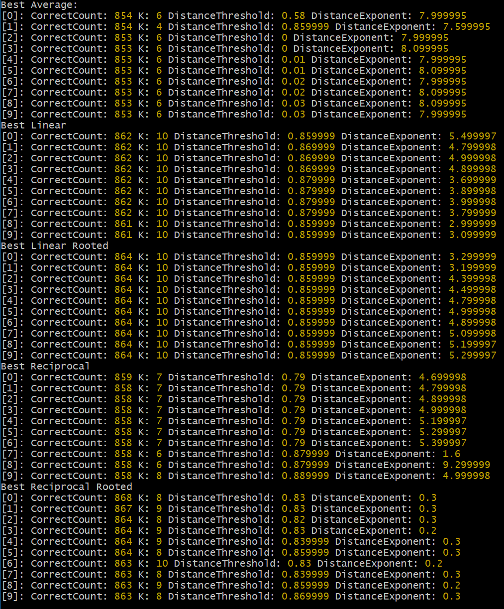
There are a few things going on in this experiment. When we compute the distance between two points, rather than using a typical Euclidean distance, we are free to modify the exponent each component difference is raised to, i.e., (|b - a|)^exponent, including fraction exponents. This exponent value is represented on the x-axis of each heatmap. Then when we compute the first portion of the distance, i.e., |b - a|, we can use a clipping threshold to essentially ignore any absolute differences between a certain value. The concept here being that very small difference will add up, but may be insignificant noise. This clipping threshold is represented on the y-axis of each heatmap (noting that the dataset has been 0->1 normalized, thus the maximum absolute difference is 1.0). Each row represents a different K value, of 1 through 20 inclusive. Each column represents a different method of combining the K neighbours of which there are 5 total methods selected here. The first column (Average) simply takes the K neighbours, sums their outputs, and divides by K - literally a simple average. The second column (Linear) uses a weighted averaging where the weight is 1 - (distance / max distance + epsilon), importantly noting that the exponent of the distance function has dramatic effect when the distance is part of the average weighting of the output. The third column (Linear Rooted) uses the same method as Linear, except when calculating the distance the final sum is raised to the reciprocal of the exponent, i.e., distance^(1/exponent). The fourth column (Reciprocal) also uses a weighted averaging, but the weight is calculated as 1 / (distance + epsilon), a more common KNN algorithm. Finally, the fifth column (Reciprocal Rooted) is the same as Reciprocal, except again the distance is raised to the reciprocal of the exponent.

Although I was skeptical about the usefulness of thresholding, it does appear to favor when all absolute component differences are ignored except for the largest and next to largest, almost akin to if the data had been binarized, but with slightly more precision still available. This specific behavior likely does not carry to other datasets, since MNIST is made of handwritten strokes which almost always peak in value, or fall just under the peak near the edges of the stroke. The efficacy of this technique should not be ignore though, as it may be useful for irking out the last few pips of accuracy in a model - though I suspect the same gain could be achieved in more clever ways of handling the data.

I did not expect the exponent choice to be so incredibly impactful, especially in the linear models which seemed to be most robust overall with respect to hyperparameters. For example in K=12 and K=13 Linear Rooted, an exponent as high as 20, if not higher showed possibly the strongest results in the entire shootout. Which begs the question, why? Larger exponents effectively penalize larger gaps between component values in terms of similarity distance. The Average and Reciprocal models also showed similar results, though they proved to be much pickier to the choice of K and exponent combination, which a narrower window of success. The Linear models may be more forgiving as the distances are essentially neighbour-normalized, rather than unbounded such as 1/distance which can explode or vanish in either direction if not correctly dialed in. The flat Average did okay, though the lack of weighting makes them weaker approximators in general especially in a spare high dimensional space like MNIST.

A small note about the Linear K=1 models, since they normalize against the max neighbour distance, but there is only 1 neighbour, the weight is effectively 1/epsilon for the single neighbour, which single precision floats don't handle well in this context (this is an expected occurence as K>1 is expected here).